PyTuxKart Ice-Hockey Game
Playing PyTuxKart Ice-Hockey Game with Image-Based Agent
Introduction
The task for this project is to program a SuperTuxKart ice-hockey player with the choice of either image-based agent or state–based agent. The objective of this hockey game is to score as many goals as possible in this 2 vs 2 tournament against the TA agents. We decided to build an image-based agent that takes the image as input and predicts the location of the puck and goal with two slightly different methods: The Pointer Method and The Heatmap Method. The reason we chose to use an image-based agent because we have been learning and processing the image with the model throughout the class. The project code repository is located at https://github.com/nez0b/ice-hockey
Image Based Agent
The primary task for an image-based agent is to design a model that takes a player image as input and infer (1) whether targets (the puck and goals) are in the image (2) the location of the puck and goals. We proposed two methods that output the above information:
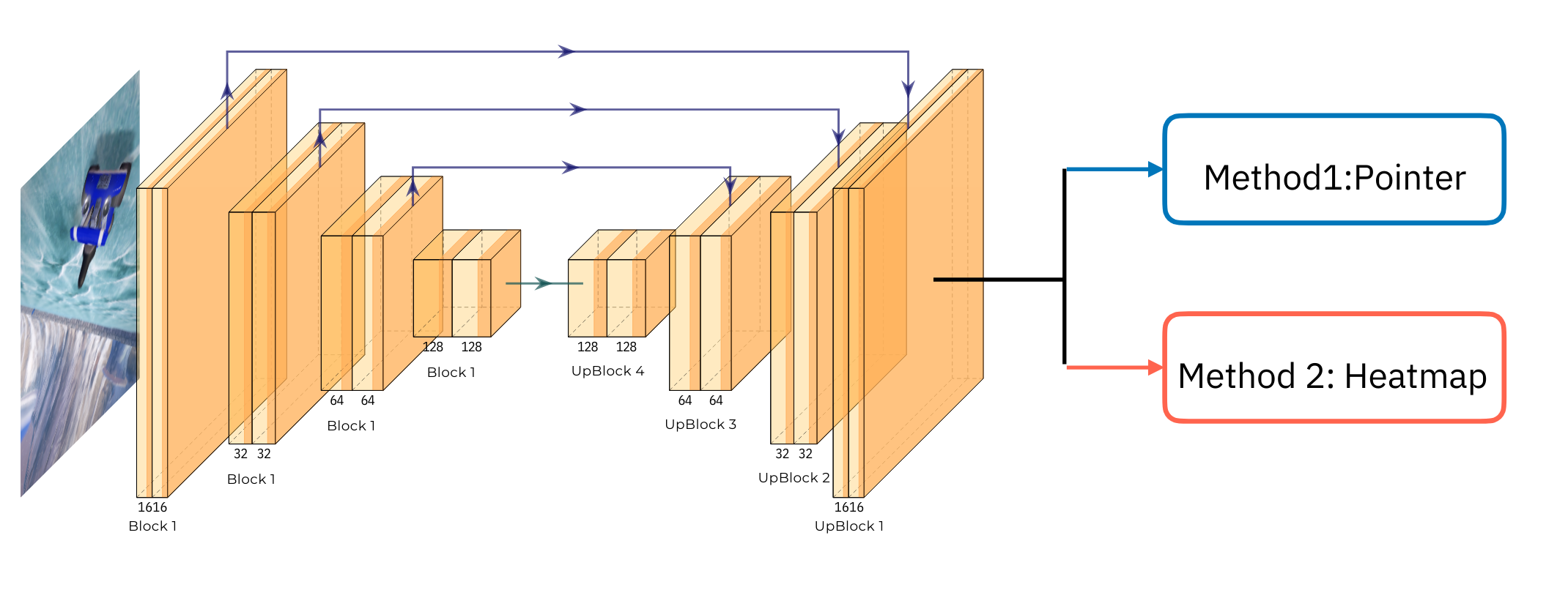
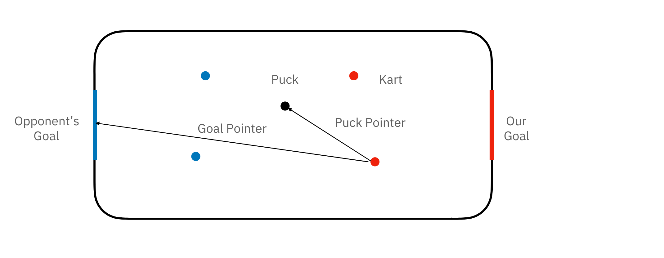
- Method 1 (The Pointer Method): The agent takes an input image and output two 2d pointer vectors of the puck and the (opponent’s) goal location. See Figure.1 for the schematic plot. With the 2d pointer vectors, the controller and calculate the distance and the angles to the puck and the goal and drives the kart to these two positions.
- Method 2 (The Heatmap Method): The agent performs a object-detection task by learning the heatmap of the input image and infer the object locations and size.
Model Architecture
For each method, we preprocess the image data and learn the features using the same model architecture. We use a Fully Convolutional Network (FCN) with each individual blocks that use residual connections to avoid vanishing gradients. The architecture first uses four down-convolutional blocks where each block has two 3x3 convolutions followed by batch normalization and ReLU. Next, the architecture uses four up-convolutions to upscale the feature map back to the original dimension. Furthermore, we use skip connections between each pair of down-convolution and up-convolution to preserve the spatial information. Finally we connect this FCN to two different final layers that will output the desired shape for each methods. See Figure.1 for a schematic plot of the model architecture. Next we discuss the details for these final layers.
Method 1: Pointer
In method 1, we connect the FCN network to a convolutional layer with four channels, which correspond to $(x_p, y_p, x_g, y_p)$, the x and y component of the pointer vectors from the kart to the puck (or the goal).
Method 2: Heatmap
In method 2, we adapt the code from HW4 and connect the FCN network to a convolutional layer with five channels. The first three channels corresponds to the heatmaps for the puck and the two goal. The last channel corresponds to the size of the detections.
Loss Function
The loss function for the method 1 network is the MSELoss between the network output $(x_p, y_p, x_g, y_g)$ and the true label:
The loss function for the method 2 network is a combination of heatmap detection loss and the object size loss:
\[l_{\text{method 2}} = \text{BCELogitLoss()} + \text{(size weight)*MSELoss()}\]To balance the heatmap and the size of the object, we choose the \textit{size weight} to be $\approx 0.0001$.
Training Data Collection
We collect the gameplay data using the given tournament/runner.py script. For example, we execute python -m tournament.runner AI AI -s ai_ai.pkl -f 5000 to collect a game play between two “AI” agents and limit the number of frames to 5000 and save it to a pickle file.
Method 1
In method 1, for each image we calculate the pointer vector to the puck location (defined by $x_p, y_p$) and the pointer vector to the goal location (defined by $x_p, y_p$). These numbers can be calculated from the following game state data:
- Kart Location : 3d world coordinate of the kart
- Kart Front Location: 3d world coordinate of the kart front.
- Puck Location: 3d world coordinate of the puck
- Goal Location: The center of the goal $(0, 0, \pm 64.5)$
Next the pointer function can be calculated from “Target vector - Kart vector”, where the target vector is “Puck(Goal) location - Kart Location” and the Kart vector is “Kart front - Kart Location”.
Method 2
For method 2, we calculate the true object location and size on the 2d projection view of the player. The conversion from a 3d world coordinate to the 2d projection view is given by:
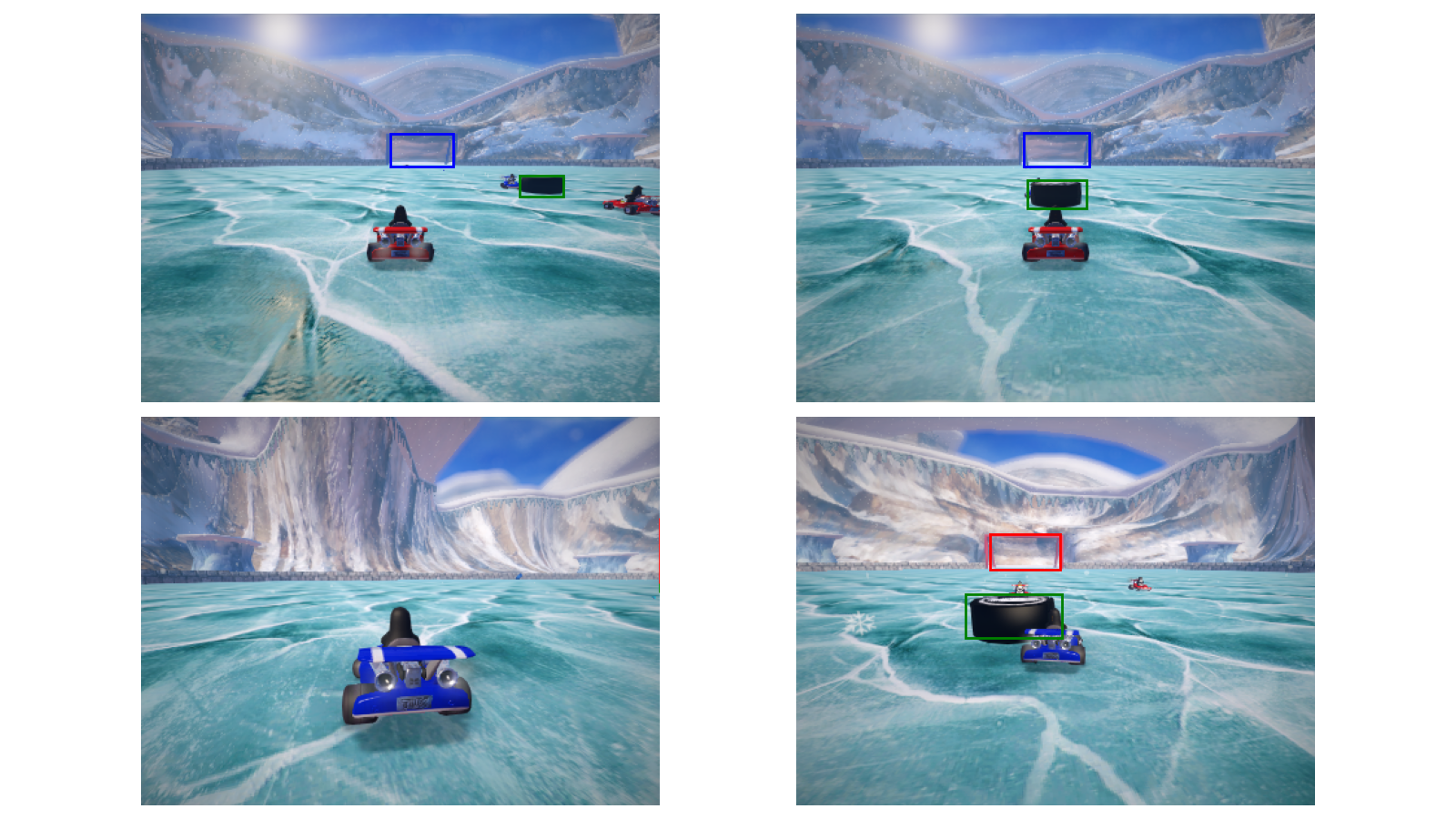
\[x_{2d} = \mathcal{V}\cdot \mathcal{P} \cdot [x_{3d}, 1]^T\]Here $\mathcal{P}$ is the 4d projection matrix, $\mathcal{V}$ is the 4d view matrix. $x_{3d}$ is the 3d world coordinate of an object. Finally the first two entries of $x_{2d}$ would be the x and y coordinate of the object projection. Given this formula we can calculate the location and the bounding boxes of the object in player’s view. See Figure.2 for an example of the object location and size.
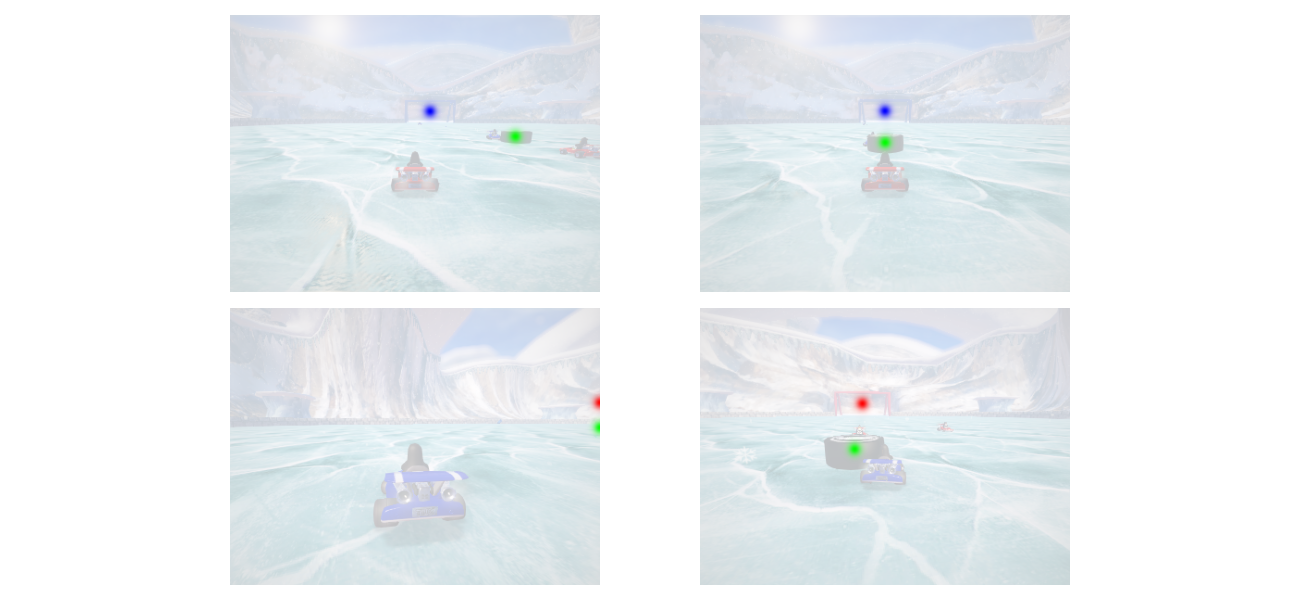
Next we take the object location and size, and convert them to the heatmap using the detection_to_heatmap function in the code. See Figure.3 for an example heatmap.
Controller Design
Method 1
Given the output $(x_p, y_p, x_g, y_g)$ of the network, we can calculate the distance and the angle to the puck and the goal. The controller algorithm works as follows:
- if the distance to the puck is larger the size of the puck, we drive the kart to the puck
- After reaching the puck, we drive the kart toward the goal location.
Method 2
The output of the network in method 2 is a heatmap that detects the locations and the size of the puck and the goals. Next, we use extract_peak function from HW4 to find the locations of the puck and the goal on the 2d player’s view. With these information, we can infer (1) whether or not the object is in the player’s view (2) The 2d location of the object. Our controller logic works as follows:
- Detect if the puck is in the player’s view. If not, set the acceleration to zero and set the brake to
Trueto reverse the direction of the kart. - If the puck is in the player’s view, set the
steerto the x coordinate of the puck’s detection location. - Repeat the same player’s logic, but replace the puck detection with the goal location.
Experiment
Training
We collect the training data using the given tournament/runner.py script. We execute python -m tournament.runner AI AI -s ai_ai.pkl-f 5000 to collect the game state data of 5000 frames, which corresponds to 20000 labeled images. We also implement the image augmentation pipeline consists of randomly changing the brightness, contrast, saturation, and the hue of images to prevent over-fitting.
Evaluation Method and Result
We used the loss from each loss function and the score running against the graders as the metrics. The losses of both methods were both high, meaning the model has deviation between the predicted values and label values. Then we run these methods against the local grader and online grader. Scoring higher score on local and online grader generally indicate the method is performing better.
Result
The results are summarized in Table1. The result for Method 1 does not perform well against local and online grader, scoring 32 out of 100 against both graders. Method 2 generally performs a better job against the local grader and online grader than Method 1. We also make the agents simply run straight, with maximum acceleration and no steering. Interestingly, even though Method 2 performed better than the agent cruising straight against the local grader, the result did not reflect on the online grader. The agent that simply cruising straight with no steering performed better against the online grader, yielding the highest score which we used this as our final submission.
| Method | Local Grader | Online Grader |
|---|---|---|
| Method 1 | $32 \%$ | $32 \%$ |
| Method 2 (First attempt) | $47 \%$ | $12 \% $ |
| Method 2 (Second attempt) | $44 \%$ | $38 \%$ |
| Agent cruising straight (First attempt) | $40 \%$ | $44 \%$ |
| Agent cruising straight (Second attempt) | $40 \%$ | $51 \%$ |
Table 1 Scores of each method against local and online grader
Alternative Method
The results of both the methods do not perform as intended and score below $70 \%$. However, instead of coming up with a completely different approach as alternative, our team suggest that the heatmap method is feasible and could performed better if we can improve in the following areas:
- Data collection : We can collect more game play data against different TA agents for more rounds to better train the model for detection. We can also exclude bad data and images when the kart crashes on the wall.
- Field of view : The kart’s camera is one of the challenge for this project. We can consider and conduct more research on the field of view of the kart and image in training and detecting.
- Controller strategy : We can design a better approach when the puck is not in the player’s view. For example, instead of simply reversing the direction of the kart, we can enable communication between two karts to exchange puck location.
Conclusions
Neither the pointer method nor the heatmap method performed well in this project. Both approaches scored lower than the agents that simply cruise straight with not steering against the online grader. If we can change one thing for this project, we should have spent less time working on Method 1, and spend more time to explore Method 2 where the agents can better detect the puck and goal from the heatmap, and improve the areas in data collection, field of view, and controller strategy.