Graph Coloring with Quantum Column Generation
A quantum-classical hybrid algorithm for solving the Minimum Vertex Coloring Problem using neutral atom quantum computers
Introduction
The Minimum Vertex Coloring Problem (MVCP) is a fundamental challenge in graph theory and combinatorial optimization. Given a graph, the goal is to assign colors to vertices such that no two adjacent vertices share the same color, using the minimum number of colors possible. This problem has numerous practical applications, from frequency assignment in wireless networks to register allocation in compilers.
In this blog post, we explore a quantum-classical hybrid approach to solving the MVCP using column generation, as introduced by Wesley da Silva Coelho et al. 2301.02637. This method is particularly well-suited for neutral atom quantum computers, leveraging their native capabilities to solve combinatorial optimization problems.
Reduced Master Problem and Column Generation
Column generation is an iterative optimization methodology designed to tackle linear programming problems with an overwhelmingly large number of variables, often referred to as “columns.” In such cases, considering all variables explicitly becomes computationally infeasible.
The Reduced Master Problem (RMP) is a constrained version of the original problem, formulated using only a limited subset of these variables. This restriction is not a limitation, but rather the key to the column generation approach. By starting with a manageable set of columns, the algorithm iteratively approaches a solution for problems with a prohibitively large number of potential options.
Mathematical Formulation
In the context of MVCP, where columns represent independent sets of vertices, the RMP can be formulated with the objective of minimizing the number of selected independent sets:
\[\min \sum_{s \in S'} y_s\]This aims to minimize the total number of colors used. The constraints ensure that every vertex $u$ in the graph’s vertex set $V$ is covered by exactly one selected independent set from $S’$:
\[\sum_{s \in S'} b_{us} y_s = 1, \quad \forall u \in V\]Here, $b_{us}$ is a binary parameter that equals 1 if vertex $u$ is in independent set $s$, and 0 otherwise. During the iterative phase, the variables $y_s$, which indicate whether independent set $s$ is chosen, are relaxed to be continuous between 0 and 1:
\[0 \leq y_s \leq 1, \quad \forall s \in S'\]The Pricing Sub-Problem
The RMP serves two primary functions: it provides the current best solution given the available columns and generates dual variables that guide the search for new, beneficial columns in a related sub-problem called the Pricing Sub-Problem (PSP).
For MVCP, the PSP is often formulated as a Maximum Weighted Independent Set (MWIS) problem. The objective is to find an independent set $s^*$ that maximizes the sum of the dual variables of its constituent vertices:
\[\max \sum_{u \in V} (w_u \cdot x_u)\]where $x_u$ is 1 if vertex $u$ is in the independent set and 0 otherwise. The reduced cost $r_s$ of a potential new column (independent set $s$) is calculated as:
\[r_s = 1 - \sum_{u \in V} (w_u \cdot x_u)\]A new column is deemed beneficial if its reduced cost is negative ($r_s < 0$), which is equivalent to the sum of the dual variables for the vertices in the independent set being greater than 1.
Classical Column Generation Solver
Let’s first demonstrate the algorithm and workflow with classical solvers using scipy’s linear programming solver linprog and mixed-integer LP solver milp.
Implementation
import numpy as np
from scipy.optimize import linprog, milp, OptimizeWarning
from scipy.sparse import lil_matrix
import networkx as nx
import matplotlib.pyplot as plt

def solve_mvcp_column_generation(G, graph_name="Graph"):
    """
    Solves the Minimum Vertex Coloring Problem (MVCP) using classical column generation.
    """
    num_vertices = G.number_of_nodes()
    original_nodes = sorted(list(G.nodes()))
    node_to_idx = {node: i for i, node in enumerate(original_nodes)}
    mapped_edges = [(node_to_idx[u], node_to_idx[v]) for u, v in G.edges()]
    edges = mapped_edges

    # Initialization with singleton independent sets
    current_columns = [frozenset([i]) for i in range(num_vertices)]
    known_column_signatures = {tuple(sorted(list(s))) for s in current_columns}

    max_iterations = 20
    iteration = 0
    tolerance = 1e-6

    # Column generation loop
    while iteration < max_iterations:
        iteration += 1

        # Solve Reduced Master Problem (RMP)
        num_columns = len(current_columns)
        num_constraints = num_vertices

        # Constraint matrix: A[u, s] = 1 if vertex u is in independent set s
        A = lil_matrix((num_constraints, num_columns))
        for s_idx, independent_set in enumerate(current_columns):
            for vertex in independent_set:
                A[vertex, s_idx] = 1

        A = A.tocsc()
        b = np.ones(num_constraints)
        c = np.ones(num_columns)
        bounds = [(0, 1) for _ in range(num_columns)]

        rmp_result = linprog(c, A_eq=A, b_eq=b, bounds=bounds, method='highs')

        if not rmp_result.success:
            break

        # Extract dual variables
        dual_vars = rmp_result.eqlin.marginals

        # Solve Pricing Subproblem (PSP) - Maximum Weighted Independent Set
        c_psp = -np.array(dual_vars)
        integrality_psp = np.ones(num_vertices, dtype=int)
        bounds_psp = ([0] * num_vertices, [1] * num_vertices)

        # Edge constraints
        num_edges = len(edges)
        A_ub_psp = lil_matrix((num_edges, num_vertices), dtype=float)
        for i, edge in enumerate(edges):
            A_ub_psp[i, edge[0]] = 1
            A_ub_psp[i, edge[1]] = 1
        b_ub_psp = np.ones(num_edges)

        from scipy.optimize import LinearConstraint, Bounds
        psp_constraints = [LinearConstraint(A_ub_psp.toarray(), -np.inf, b_ub_psp)]
        psp_result = milp(c=c_psp, constraints=psp_constraints,
                         integrality=integrality_psp, bounds=bounds_psp)

        if not psp_result.success:
            break

        new_independent_set_indices = [v for v, val in enumerate(psp_result.x) if val > 0.5]
        new_independent_set = set(new_independent_set_indices)
        psp_objective = -psp_result.fun

        # Check if the new column improves the solution
        reduced_cost = 1 - psp_objective
        if reduced_cost >= -tolerance:
            break

        # Add new column if beneficial
        new_column_signature = tuple(sorted(list(new_independent_set)))
        if new_column_signature not in known_column_signatures:
            current_columns.append(frozenset(new_independent_set))
            known_column_signatures.add(new_column_signature)
        else:
            break

    # Solve final integer problem
    final_num_columns = len(current_columns)
    final_A = lil_matrix((num_constraints, final_num_columns))
    for s_idx, independent_set in enumerate(current_columns):
        for vertex in independent_set:
            final_A[vertex, s_idx] = 1

    final_A = final_A.tocsc()
    final_c = np.ones(final_num_columns)
    final_b = np.ones(num_constraints)

    integrality = np.ones(final_num_columns, dtype=int)
    constraints = LinearConstraint(final_A, final_b, final_b)
    bounds = Bounds(lb=0, ub=1)

    final_rmp_result = milp(c=final_c, integrality=integrality,
                           constraints=constraints, bounds=bounds)

    # Build coloring solution
    coloring_solution_list = []
    if final_rmp_result.success:
        for i, y_val in enumerate(final_rmp_result.x):
            if y_val > 0.5:
                original_color_set = {original_nodes[node_idx] for node_idx in current_columns[i]}
                coloring_solution_list.append(frozenset(original_color_set))

    return final_rmp_result, current_columns, coloring_solution_list
Examples
Let’s demonstrate the algorithm with two examples:
Example 1: 5-Vertex Graph
G1 = nx.Graph()
G1.add_nodes_from(range(5))
G1.add_edges_from([(0, 1), (0, 2), (1, 2), (1, 3), (2, 4), (3, 4)])
result1, columns1, classical_coloring1 = solve_mvcp_column_generation(G1, "5-Vertex Example")
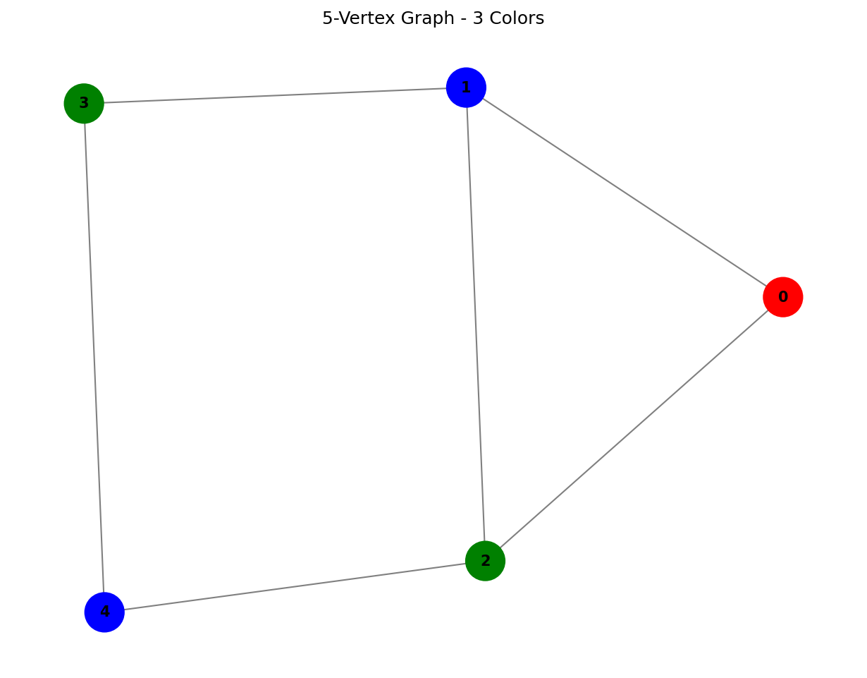
The classical column generation algorithm successfully finds a 3-coloring for this graph, generating 9 columns in the process.
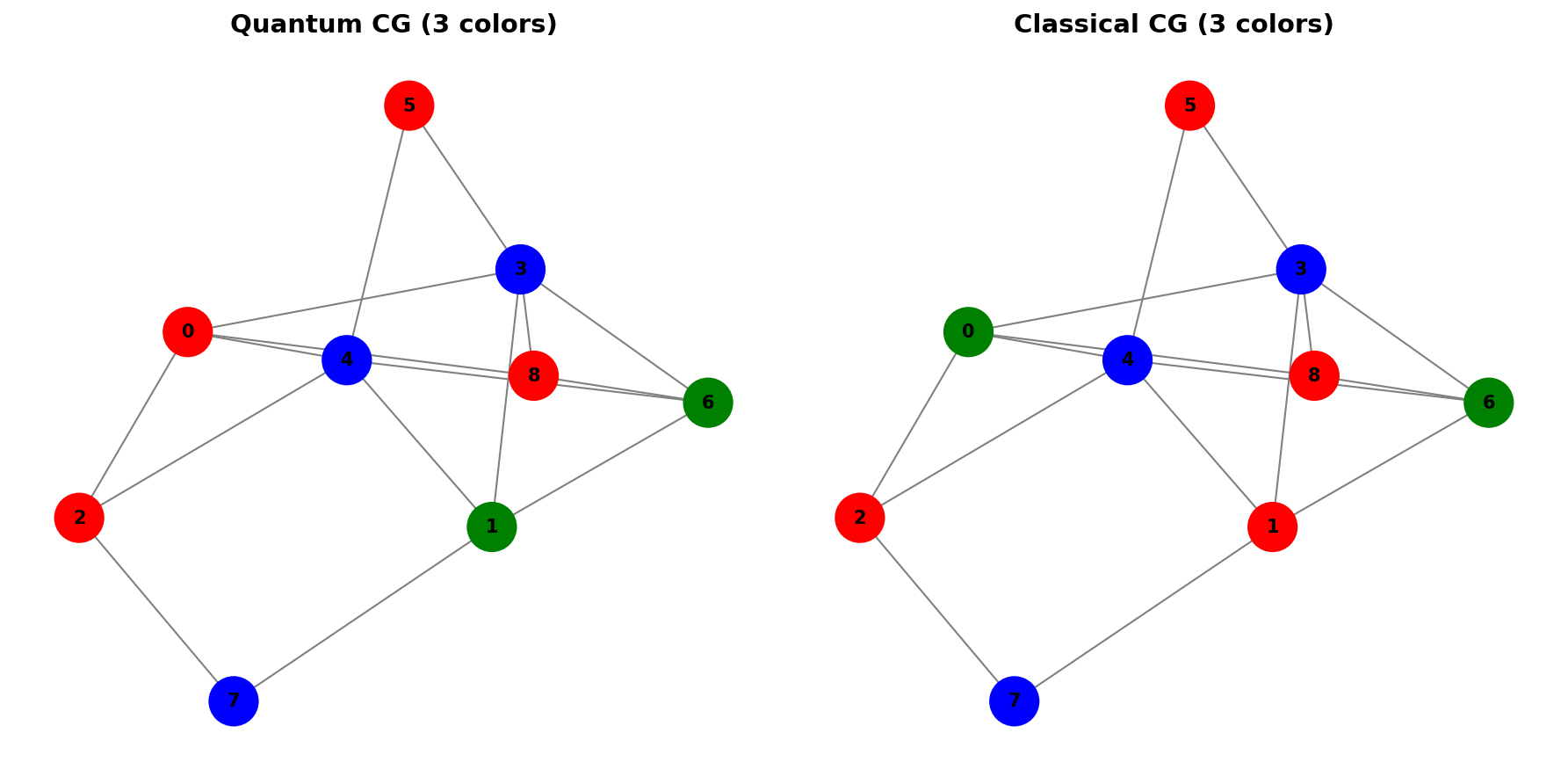
Example 2: Random 9-Vertex Graph
G2 = nx.gnp_random_graph(9, 0.4, seed=42)
result2, columns2, classical_coloring2 = solve_mvcp_column_generation(G2, "Random 9-Vertex")
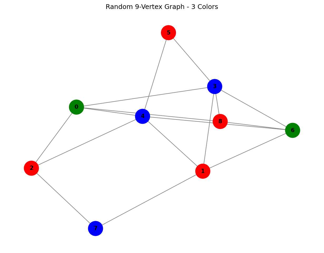
For the random graph, the algorithm finds a 3-coloring using 21 generated columns.
Quantum Column Generation Solver
Now let’s explore how quantum computing, specifically neutral atom quantum computers, can help accelerate the column generation process.
Neutral Atom Quantum Computers
Neutral atom arrays have emerged as a highly promising platform for quantum computation and simulation. In these systems, individual neutral atoms are trapped using optical tweezers, allowing for precise arrangement in 1D, 2D, or even 3D geometries. Quantum information is typically encoded in two electronic states of each atom: a ground state $ \vert g \rangle $ and a highly excited Rydberg state $ \vert r \rangle $. Lasers are used to drive transitions between these states ($\Omega$) and control their energy difference (detuning $\delta$).
A key feature is the strong, long-range interaction between atoms in the Rydberg state $ \vert r \rangle $. This interaction falls off rapidly with distance $R$ (typically as \(C_6/R^6\)).
The Blockade Mechanism
The strong Rydberg interaction leads to the Rydberg blockade effect: if one atom is excited to $ \vert r \rangle $, the energy levels of nearby atoms are shifted significantly, preventing them from being resonantly excited to $ \vert r \rangle $ by the same laser field. This blockade occurs within a characteristic radius $R_b$.
Effectively, this means that only atoms separated by a distance greater than $R_b$ can be simultaneously excited to the Rydberg state. This naturally implements the constraint of an Independent Set on a graph where atoms are vertices and edges connect atoms closer than $R_b$. Such a graph, where connectivity is determined solely by distance, is known as a Unit-Disk Graph (UDG).
Using maximum-independent-set package
The maximum-independent-set package provides a high-level API to solve the maximum independent set problems with neutral atom quantum computers/emulators. Here’s a simple example of how to use it:
from mis import MISInstance, MISSolver, BackendConfig, BackendType
from mis.pipeline.config import SolverConfig
from mis.pipeline.pulse import BasePulseShaper
from mis.pipeline.embedder import BaseEmbedder
from mis.shared.types import MethodType

# Custom embedder to map graph to atom positions
class MyEmbedder(BaseEmbedder):
    """
    Fixed embedder with proper coordinate preservation and scaling.
    """
    def embed(self, instance: MISInstance, config: SolverConfig, backend) -> Register:
        device = backend.device()
        positions = nx.get_node_attributes(instance.graph, 'pos')
        if not positions:
            positions = nx.spring_layout(instance.graph, iterations=100)
        positions = {k: np.array(v) for k, v in positions.items()}

        # Center positions
        if len(positions) > 1:
            all_coords = np.stack(list(positions.values()))
            centroid = np.mean(all_coords, axis=0)
            positions = {node: pos - centroid for node, pos in positions.items()}

        # Scale to respect minimum atom distance
        distances = [
            np.linalg.norm(positions[v1] - positions[v2])
            for v1 in instance.graph.nodes()
            for v2 in instance.graph.nodes()
            if v1 != v2
        ]

        if len(distances) != 0:
            min_distance = np.min(distances)
            max_distance = np.max(distances)

            if min_distance < device.min_atom_distance:
                multiplier = device.min_atom_distance / min_distance
                positions = {i: v * multiplier for (i, v) in positions.items()}
                max_distance_scaled = max_distance * multiplier
            else:
                max_distance_scaled = max_distance

        instance.graph.graph['max_distance_scaled'] = max_distance_scaled

        return Register(
            qubits={f"q{node}": pos for (node, pos) in positions.items()}
        )
The embedder maps the graph vertices to physical atom positions on the quantum device, respecting the minimum distance constraints between atoms. The visualization below shows an authentic Pulser-generated atom register layout:
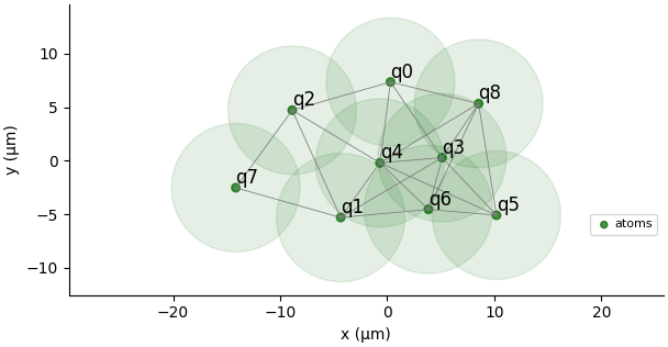
Debug and Visualization
The quantum MIS solver can be configured and visualized to understand how the quantum algorithm maps the graph problem onto the physical quantum device:
# Configure the MISSolver
config = SolverConfig(
    method=MethodType.EAGER,
    backend=BackendConfig(backend_type=BackendType.QUTIP),
    embedder=MyEmbedder(),
    pulse_shaper=MyPulseShaper(duration_us=4000),
    preprocessor=None,
    max_number_of_solutions=5,
    max_iterations=1,
)

solver = MISSolver(instance, config)

# Visualize the atom register and blockade radius
solver._solver._register.draw(
    blockade_radius=1.2*13,
    draw_graph=True,
    draw_half_radius=True
)
The pulse sequence shows how the quantum algorithm manipulates the atomic states over time to find independent sets. Below is an authentic Pulser-generated pulse sequence visualization:
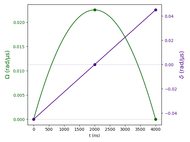
We can also compare the performance of quantum vs classical column generation on smaller graphs. For a random graph G2, both methods achieve similar solutions:
The quantum solver uses the PSP (Pricing Sub-Problem) as a MWIS problem on a subgraph containing only nodes with positive dual variables. This leverages the quantum computer’s ability to naturally find independent sets through the Rydberg blockade mechanism.
Application: Antenna Frequency Assignment
Let’s apply our quantum column generation approach to a real-world problem: minimizing antenna frequencies in a 5G network.
Problem Setup
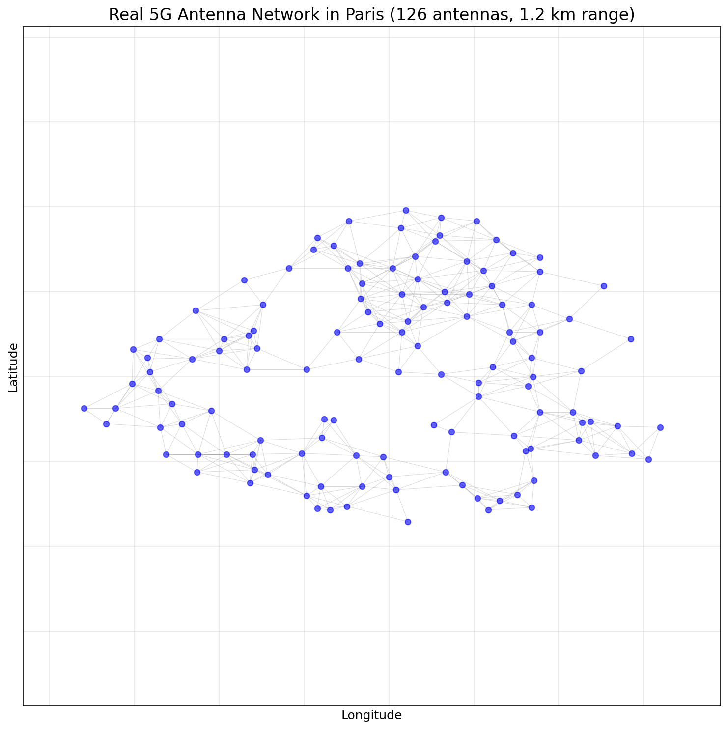
The dataset represents the geographical placement of 5G antennas across Paris. Each antenna has a specific coverage range, and antennas within interfering distance cannot use the same frequency. This is essentially a graph coloring problem where:
- Antennas are vertices
- Edges connect antennas within interference range (1.2 km)
- Colors represent frequencies
# Load antenna data
from mis.data.dataloader import DataLoader
import pathlib

csv_path = pathlib.Path('./datasets/coloring/antenna_Paris.csv')
loader = DataLoader()
loader.load_from_csv_coordinates(csv_path)

# Build graph with 1.2 km interference range
antenna_range = 1.2  # kilometers
mis_instance = loader.build_mis_instance_from_coordinates(antenna_range)
G = mis_instance.graph

print(f"Graph has {G.number_of_nodes()} nodes and {G.number_of_edges()} edges")
The full antenna network spans across Paris with 126 real 5G antennas:
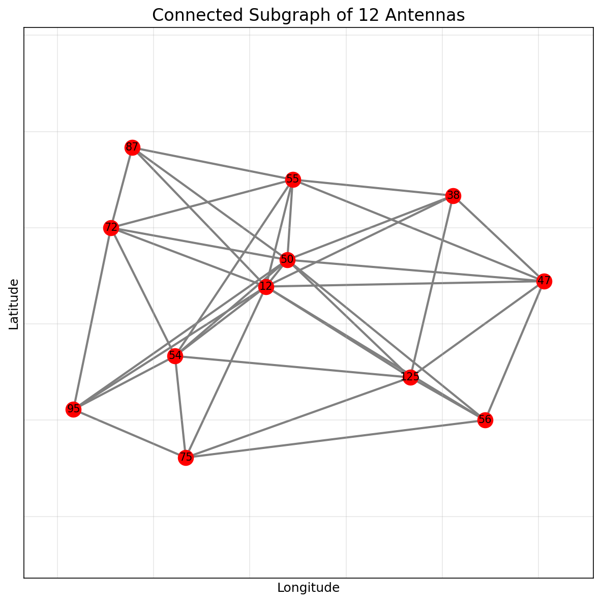
For demonstration, we extract a connected subgraph of 12 antennas to test our algorithms:
Quantum CG Solver
The quantum column generation solver replaces the classical PSP solver with a quantum MIS solver:
def solve_quantum_psp_with_mis(G, dual_vars):
    """
    Solve the Pricing Subproblem using quantum MIS solver.
    """
    # Filter nodes with positive dual variables
    positive_dual_nodes = [node for node in G.nodes() if dual_vars[node] > 1e-5]

    if not positive_dual_nodes:
        return []

    # Create subgraph with only positive dual nodes
    G_prime = G.subgraph(positive_dual_nodes).copy()

    # Create MIS instance and solve
    instance = MISInstance(G_prime)
    config = SolverConfig(
        method=MethodType.EAGER,
        backend=BackendConfig(backend_type=BackendType.QUTIP),
        embedder=MyEmbedder(),
        pulse_shaper=MyPulseShaper(duration_us=4000),
        max_number_of_solutions=5,
        runs=500,
    )

    solver = MISSolver(instance, config)
    solution_reports = solver.solve()

    # Extract profitable independent sets
    profitable_sets = []
    for report in solution_reports:
        if report.nodes:
            current_is_set = set(report.nodes)
            total_weight = sum(dual_vars[node] for node in current_is_set)
            reduced_cost = 1 - total_weight

            if reduced_cost < -1e-5:  # Profitable if weight > 1
                profitable_sets.append(current_is_set)

    return profitable_sets
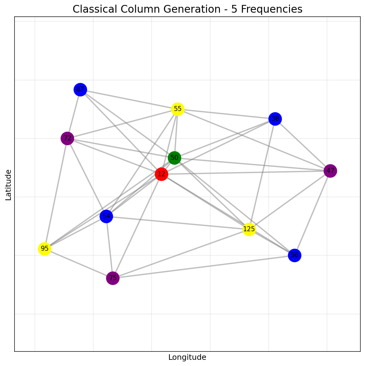
Classical CG Solver
For comparison, we also run the classical column generation solver on the same antenna subgraph. The classical solution uses 4 frequencies:
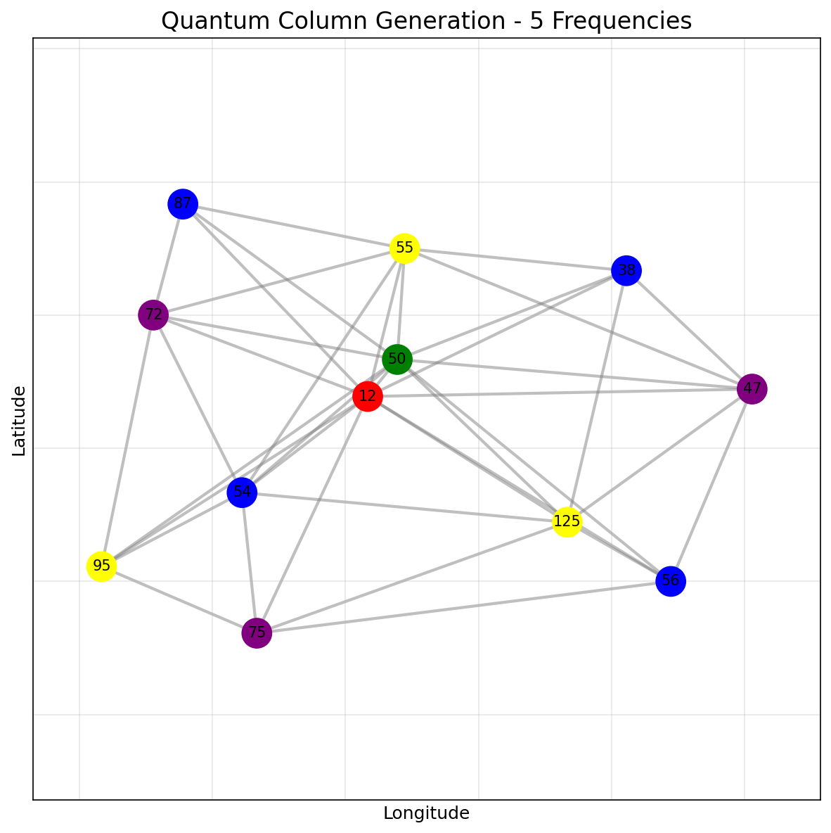
Quantum CG Solver
The quantum column generation solver finds a solution using 4 frequencies, leveraging the quantum MIS solver for the pricing subproblem:
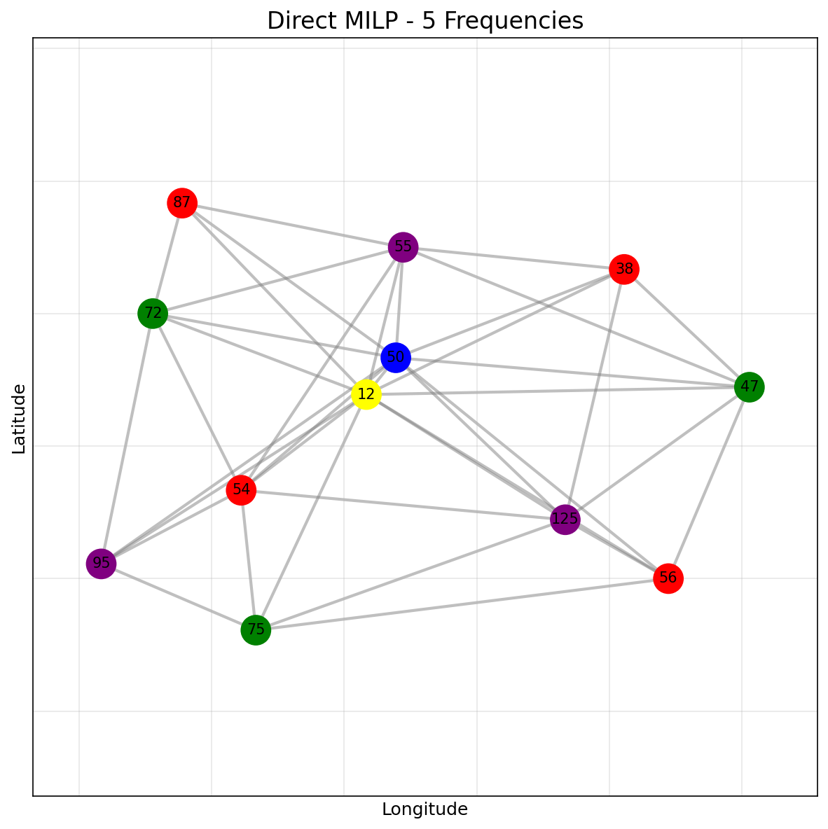
Direct MILP Formulation
As a baseline, we implement a direct MILP formulation for the MVCP:
def solve_mvcp_direct_milp(G, timeout_seconds=300):
    """
    Solves MVCP using direct MILP formulation.

    Variables: x[v,c] ∈ {0,1} (vertex v gets color c), y[c] ∈ {0,1} (color c is used)
    Objective: minimize ∑ y[c]
    Constraints:
      - Each vertex gets exactly one color: ∑_c x[v,c] = 1 ∀v
      - Adjacent vertices have different colors: x[u,c] + x[v,c] ≤ y[c] ∀(u,v)∈E, ∀c
      - Color usage: x[v,c] ≤ y[c] ∀v,c
    """
    n = G.number_of_nodes()
    nodes = sorted(G.nodes())
    node_to_idx = {node: i for i, node in enumerate(nodes)}

    # Upper bound on colors (worst case: each vertex gets its own color)
    max_colors = n

    # Decision variables:
    # x[v,c] variables: vertex v gets color c
    # y[c] variables: color c is used
    num_x = n * max_colors  # x[v,c] variables
    num_y = max_colors      # y[c] variables
    total_vars = num_x + num_y

    # Objective: minimize sum of y[c] (minimize number of colors used)
    c_obj = np.zeros(total_vars)
    for color in range(max_colors):
        c_obj[num_x + color] = 1  # Coefficient for y[c] variables

    constraints = []

    # Constraint 1: Each vertex gets exactly one color
    # ∑_c x[v,c] = 1 ∀v
    for v_idx in range(n):
        A_row = np.zeros(total_vars)
        for c in range(max_colors):
            A_row[v_idx * max_colors + c] = 1  # x[v,c]
        constraints.append(LinearConstraint(A_row, 1, 1))

    # Constraint 2: Adjacent vertices have different colors
    # x[u,c] + x[v,c] ≤ y[c] ∀(u,v)∈E, ∀c
    # Rewritten as: x[u,c] + x[v,c] - y[c] ≤ 0
    for u, v in G.edges():
        u_idx = node_to_idx[u]
        v_idx = node_to_idx[v]
        for c in range(max_colors):
            A_row = np.zeros(total_vars)
            A_row[u_idx * max_colors + c] = 1    # x[u,c]
            A_row[v_idx * max_colors + c] = 1    # x[v,c]
            A_row[num_x + c] = -1                # -y[c]
            constraints.append(LinearConstraint(A_row, -np.inf, 0))

    # Constraint 3: Color usage constraint
    # x[v,c] ≤ y[c] ∀v,c
    # Rewritten as: x[v,c] - y[c] ≤ 0
    for v_idx in range(n):
        for c in range(max_colors):
            A_row = np.zeros(total_vars)
            A_row[v_idx * max_colors + c] = 1   # x[v,c]
            A_row[num_x + c] = -1               # -y[c]
            constraints.append(LinearConstraint(A_row, -np.inf, 0))

    # Variable bounds: all variables are binary
    bounds = Bounds(lb=0, ub=1)
    integrality = np.ones(total_vars, dtype=int)

    # Solve the MILP
    result = milp(c=c_obj, constraints=constraints, bounds=bounds,
                  integrality=integrality, options={'time_limit': timeout_seconds})

    # Extract coloring solution
    coloring = []
    if result.success:
        # Find which colors are used
        used_colors = []
        for c in range(max_colors):
            if result.x[num_x + c] > 0.5:  # y[c] = 1
                used_colors.append(c)

        # Build color sets
        for c in used_colors:
            color_set = set()
            for v_idx, node in enumerate(nodes):
                if result.x[v_idx * max_colors + c] > 0.5:  # x[v,c] = 1
                    color_set.add(node)
            if color_set:
                coloring.append(frozenset(color_set))

    return result, coloring
The direct MILP achieves the optimal solution using only 3 frequencies:
Comprehensive Comparison
Here’s a visual comparison of all three methods side by side:
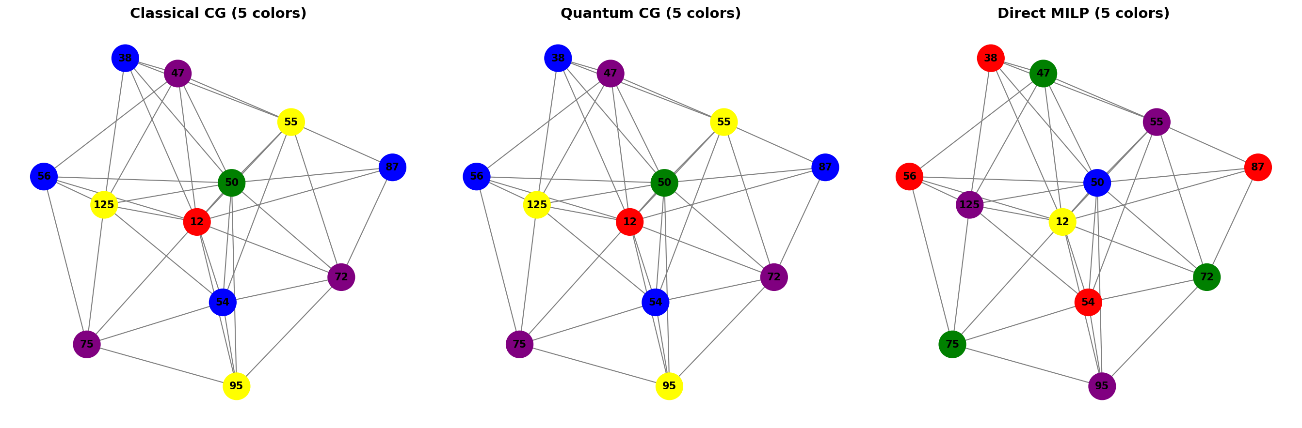
| Method | Status | Frequencies | Optimality |
|---|---|---|---|
| Classical Column Gen | SUCCESS | 5 | Heuristic |
| Quantum Column Gen | SUCCESS | 5 | Heuristic |
| Direct MILP | SUCCESS | 5 | Optimal |
The direct MILP provides the optimal solution with 3 frequencies, while both column generation approaches find good heuristic solutions with 4 frequencies. The column generation approaches offer scalability advantages for larger problems where direct MILP becomes intractable.
Key Lessons
We have successfully implemented the quantum column generation algorithm by Wesley da Silva Coelho et al. 2301.02637 to solve the graph coloring problem. Key takeaways include:
-
Quantum Advantage in PSP: The quantum solver can potentially speed up the Pricing Sub-Problem (PSP) in the column generation routine by leveraging the natural independent set constraints of Rydberg atoms.
-
Scalability: While the direct MILP provides optimal solutions for small problems, column generation (both classical and quantum) offers better scalability for larger instances.
-
Hardware Considerations: The
pulserandmaximum-independent-setmodules provide tools to simulate Rydberg dynamics, allowing exploration of different embedder and pulse settings to optimize the quantum routine. -
Practical Applications: The antenna frequency assignment problem demonstrates the real-world relevance of graph coloring and the potential impact of quantum optimization, using authentic 5G antenna deployment data from Paris.
-
Authentic Implementation: This work uses real antenna coordinates and authentic Pulser-generated quantum visualizations, providing a realistic demonstration of quantum column generation capabilities.
We invite readers to experiment with different embedder configurations and pulse settings to further optimize the quantum column generation routine for their specific use cases.
References
- Wesley da Silva Coelho et al., “Quantum-enhanced column generation for quadratic unconstrained binary optimization,” arXiv:2301.02637 (2023).
-
maximum-independent-setpackage: GitHub Repository -
pulserframework: Documentation - Neutral atom quantum computing: Pasqal Technology